Risk factors used in derivative pricing models come in two forms: observable and fitted.
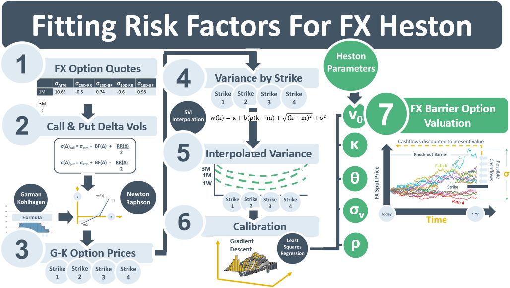
On the RH side of the diagram below are Heston model parameters used to control the simulated paths of FX spot rates. Some paths will reach the maturity of the FX barrier option the simulation is designed to value and some won’t. The ones that reach maturity will have avoided the knock-out barrier and exceeded the strike price. Their prices at maturity will be discounted to PV and averaged to determine the value of the barrier option. The Heston params determine the variance (ν) of the simulated diffusion. They also determine how that variance reverts to a mean (κ) over time and is correlated (ρ) with the underlying FX spot rate.
The Heston model params are a specific type of fitted RF. They need to be calibrated using a numerical technique (Step 6)) to another type of fitted RF, a set of interpolated variance curves. The primary unit of the Heston model is the variance, ν, of the underlying FX spot rate. Variance is easier to work with mathematically than both option prices and IV. But FX options are not quoted in variance. They are quoted in option price spreads at specific deltas and tenors. A transformation process is therefore needed to transform quoted FX option prices, the observable RFs, into the fitted variance curves.
The quoted FX option prices are the market’s view of the market risk of the FX spot rate at different maturities and strikes. The more expensive the options the more volatility assumed in the underlying FX spot rates. FX options are quoted using risk-reversal and butterfly spread instruments. These capture the tilt and skew of the volatility curves embedded in the option prices.
Step 1 in the transformation process converts the RR and BF quotes into call & put vols at specific deltas. Call and put delta vols are a more common way of representing vol – consistent with options quoted in e.g. equities markets. Steps 2 and 3 convert the call & put delta quotes into call & put vols at specific strike prices – another type of fitted RF. Step 4 converts the call and put prices for each strike into variances by strike and Step 5 converts the variances by strike into an interpolated variance curve using the SVI interpolation technique.
Step 6 calibrates the Heston parameters to the variance curve. It is using least squares regression and gradient descent to – in effect – synch the parameters back to the option market quotes in Step 1. Once calibrated, the parameters are ready to drive the Monte Carlo diffusion that will calculate the value of the barrier option.