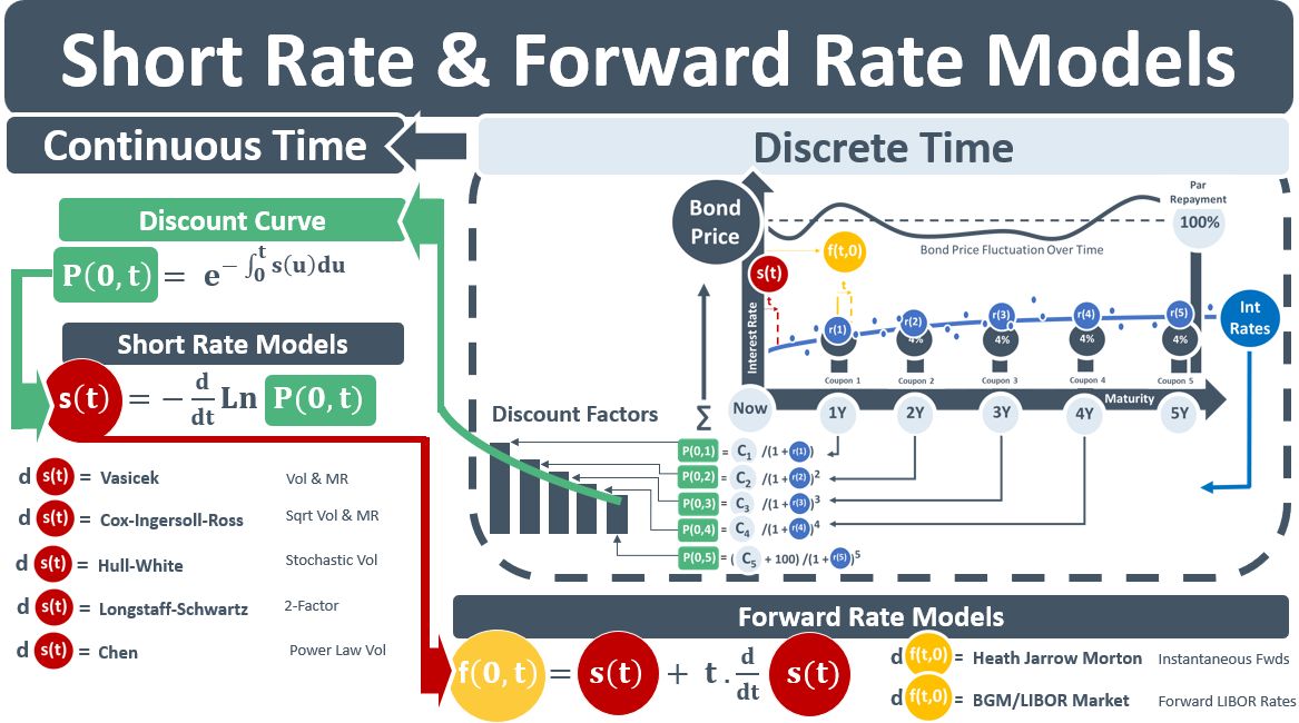
A bond is a loan. It has future CFs: its coupons, and the loan repayment. Each future CF has a PV. The PV is the amount that would have to be invested today, at the rate applicable for the period, to earn the future value, i.e. the future CF. The sum of the PVs = the valuation of the bond. The bond valuation flow in the top RH diagram below contains the formulas for the PVs [see P(0,t)] of the CFs. The formulas are based on discrete time intervals (1Y, 2Y, etc) for rates that are observable in the market.
The CFs of bonds, however, do not usually fall on dates that exactly match the dates of the discrete observable rates. A continuous curve therefore needs to be fitted to the observable rates. If the CFs are uncertain because there is optionality in bonds or derivatives’ underlying rates, then term structure models are needed which simulate how rates vary over time. The two main categories of TSMs are short rate s(t) models and fwd rate f(0,t) models. SRMs model a rate at time 0 with an instantaneous maturity. FRMs model rates that start in the future.
The concept of the PV, aka the DF, is the building block for all valuations in a bank’s trading book. Both s(t) and f(0,t) are derived from it. The top LHS eqn below shows that s(t) is the slope of the log of the PV. And the eqn at the bottom of the diagram shows that f(0,t) is derived from s(t).
TSMs are differential eqns that model the evolution of either s(t) or f(0,t) over time. See the ds(t) and df(0,t) eqns below. The first generation of TSMs modelled ds(t). E.g., Vasicek (1977) modelled the short rate using three parameters: growth rate, vol and mean-reversion. Later stochastic vol SRMs allowed the vol parameter to be random. While SRMs were easy to implement and enabled closed-form bond prices, they do not fit the observable data – neither bond prices not IR derivative prices – that they were trying to model. SRMs were trying to replicate changes in a curve that was full of fwd rates by modelling the change of a single short rate – a tall order.
With the growth of derivatives in the 1980s, researchers were incentivised to develop models that could reproduce market prices. The foundational Black-Scholes-Merton framework – in which derivative pricing models were being developed – required that derivatives were priced in a no-arbitrage market setting.
The HJM framework expanded the SRM framework to create a unifying approach that allowed curves to be built directly from FRs. Instead of trying to produce the FR curve from a single short rate – as the SRMs tried to do, HJM modelled the entire forward rate curve. Constraints were added to attempt to make the curve arbitrage-free. In the late 1990s, the LIBOR market model extended the HJM framework so that it could exactly reproduce discrete forward LIBOR rates. The LMM model became the market standard for pricing interest rate derivatives.