The first QF models were developed for equity prices. GBM & Black-Scholes modelled equities & their options. A natural extension of these models would have been models for bond prices. But this is not what happened. Bonds are issued with many maturities with varying liquidity making them difficult to build models for. But bond prices can be calculated if you know the IRs applicable for its CFs. So instead of building models for bond prices, researchers focused on models for IRs at different maturities. The models became known as term structure models.
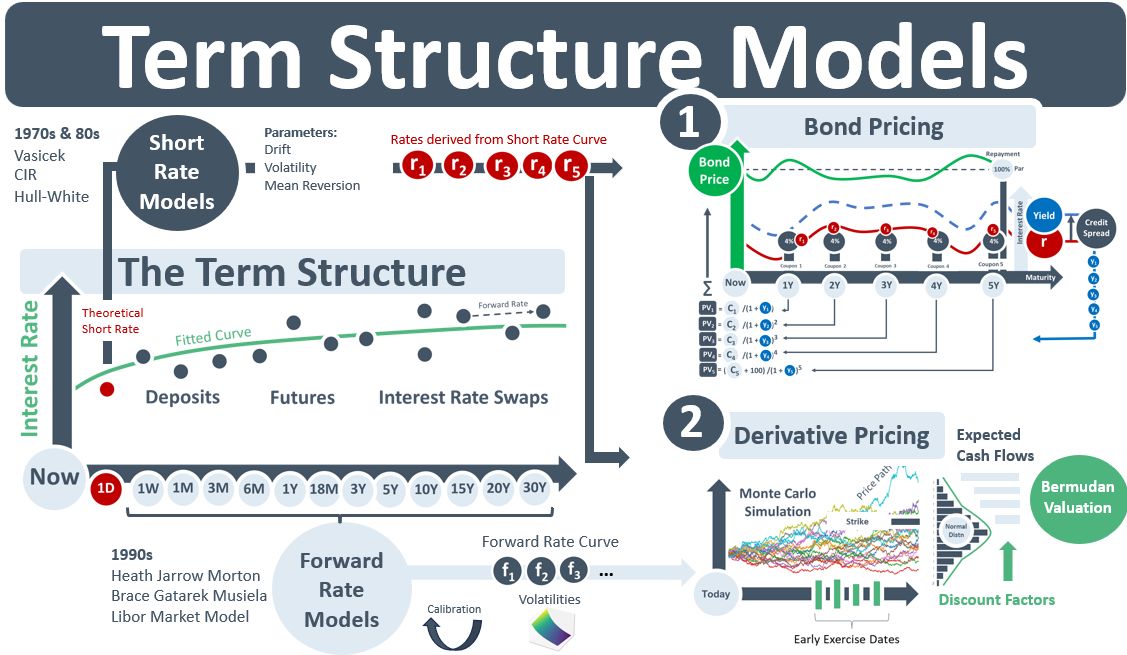
The first TSMs were the short rate models (SRMs). Vasicek, CIR and HW are examples. SRMs use parameters such as drift, volatility and mean reversion to model a short rate, equivalent to the red overnight (1D) rate in the TS diagram below, to project an IR curve that is based on assumptions about IRs in the market generally. The objective with all curve building is to closely match observable market rates. The SRMs though rarely did this as the SRM curve-building process did not take observable data as inputs. Instead, they tried to match the observable TS after the curve was built.
Once SRM-curves were built, they were used for two purposes: 1) To price illiquid bonds: The fitted, continuous curves allowed rates at any maturity to be obtained and fed into a bond pricing routine. The top RH example below shows red rates r1 to r5 being obtained from the fitted SRM curve and passed into the bond pricing eqn. to generate the price for the illiquid bond. 2) To price derivatives: The bottom RH diagram shows SRM-derived rates being fed into a MC simulation for a Bermudan swaption. Thousands of rates are simulated. They determine both the early-exercise and maturity date CFs of the Bermudan. The valuation of the Bermudan is the avg of the discounted CFs.
Money markets and derivatives trading in the 1980s and 90s led to methodology changes in curve-building. The first was that instruments such as deposits, futures, FRAs and swaps replaced bond yields as the calibrating instruments for TSMs. The second was that SRMs were replaced by a new family of TSMs called fwd rate models (FRMs). While SRMs were easy to work with mathematically, the resulting curves did not fit the observable rates very well. And the fact that they did not take the observable curve as a model input also meant that they did not take advantage of the information content of the curve. A curve has embedded fwd rates which have their own vols. The relationships btw fwd rates are captured in correlations.
The move to building FRMs whose calibration routines were able to reproduce both observable fwd rates and the vols of those fwd rates happened gradually. The HJM framework was able to reproduce the initial fwd rates but not their vols (as implied from traded caplets & swaptions). The LMM model that succeeded it was able to reproduce both the fwd rates and their vols.